As a result of a monetary policy to cool the economy, the U.S. Federal Reserve (the Fed) rapidly increased the federal funds rate which created several financing challenges within the real estate industry, and has largely contributed to a disconnect in value among willing buyers, willing sellers, and financing resources. Although the Fed recently lowered the federal funds rate by 50 basis points, the underlying disconnect has not been resolved and the following question still stands; “What is real estate worth today?” 

Real estate analysts generally use prior sales activity and current net operating income to help benchmark property value. But because of the historical rapid rise in the federal funds rate, the continued holding period of the higher federal funds rate, and the tightening of commercial real estate lending, the above disconnect remains. This has led to a scarcity of non-distressed sales and non-owner-occupier sales from which to extract relevant pricing information. Consequently, many real estate professionals are limited to mathematics and using data from an inapplicable (or incomparable) market cycle. Further, the data scarcity issue gives rise to an unhelpful practice of adjusting older and/or stale data to extract investment rate information  for a particular real estate investment. 

This article focuses on the going-in capitalization rate, which is uniquely different from a terminal or reversionary rate associated with a hypothetical exit or sale of a property at the end of a prospective hold period. The “going-in” rate is the estimated return or yield on a real estate investment, and is generally used in conjunction with a stabilized cash flow stream.  

While real estate values are the result of a combination of quantitative and qualitative inputs, deriving a market-based investment rate is one of the more critical and difficult inputs in today’s environment. With the proper methodology, a reliable estimate of rates can be identified for application in lieu of relying heavily upon past transactions. 

This article will demonstrate how the capital stack structure of a real estate investment is useful in deriving a market-oriented capitalization rate.

Capitalization rate computation methods

A capitalization rate (Cap Rate) is generally defined as the income rate for a total real property interest that reflects the relationship between a single year’s net operating income expectancy and the total property price or value. There are a variety of methods to calculate a market-oriented Cap Rate for a real property investment. This is especially helpful when there is a scarcity of comparable sales to extract Cap Rates from. 

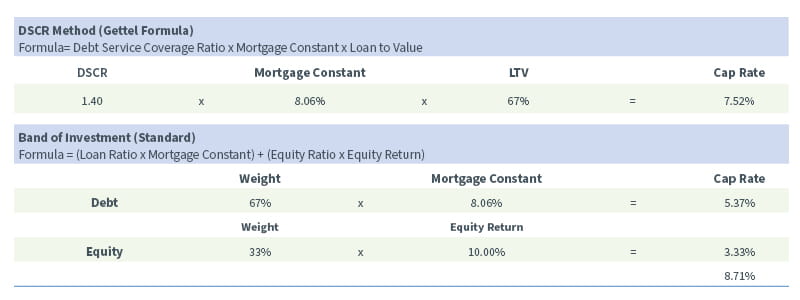
One of the earlier real estate methods known to derive a Cap Rate is credited to Wiliam MacRossie who introduced the Band-of-Investment (BOI) concept to the wider real estate profession. The BOI method captures the real estate investment’s mortgage and equity components to derive a weighted average Cap Rate. However, the BOI method does not incorporate mortgage amortization, changes in property value, or any build-up of equity. Because of these constraints, the BOI, when not employed correctly, may undervalue the real estate investment, and is why alternative Cap Rate methods should be considered and/or used in conjunction with the BOI. 

Some alternative methods that can be used to estimate the Cap Rate, beyond the BOI, include the Ellwood formula, Ackerson formula, and Gettel formula.

Methods explained

Ellwood Formula: This method effectively “builds up” a Cap Rate by looking at mortgage and equity requirements, and is otherwise known as a “mortgage-equity” analysis. The function of this formula allows a preparer to analyze how financing terms impact real estate value, and is different from the BOI method because it relies heavily on financing terms.

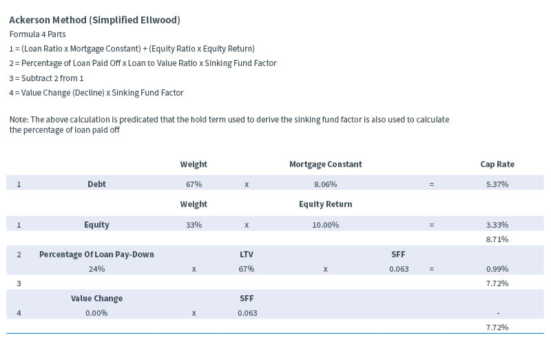
Ackerson Formula: This method is considered to be a simplified Ellwood Formula, commonly known as “Ellwood without Algebra”, and effectively blends an equity yield and mortgage terms, including both interest and amortization. The weighted average total of equity and debt is reduced by any equity build-up. This is done by adding a sinking fund factor to calculate the hypothetical equity build-up as well as real property maintenance and replacement considerations commonly estimated through depreciation. Both of these components would be typical over a long-term hold period. Please note that the authors of this article do not suggest the use of this method to value assets with interest-only loan terms because this type of loan structure does not provide for any equity build-up.

Further, in periods of unusually high volatility, a Value Change Factor may be added to the Ackerson method to measure the positive (value growth) or negative (value decline) market sentiment on a Cap Rate. This input is included in the Ackerson table example (See the Addenda to this article) that follows; albeit for simplicity purposes of the calculation, we did not employ it. 

Also note that this article focuses on the simplified Ellwood Formula via the Ackerson method rather than working through the more complex algebraic equations involved in the Ellwood Formula. 

Gettel Formula: This method is commonly referred to as the Debt Service Coverage Ratio Method (DSCR Method). This method uses the perspective of a lender to calculate a capitalization rate using basic mortgage terms. It is different from the Ellwood method because it simplifies the above two approaches by focusing solely on the debt components: mortgage constant, loan-to-value, and the DSCR. Because the DSCR encapsulates the property’s potential to generate cash flow after servicing a loan, it considers the return of capital to the equity owner. An investor’s rate of return on its investment (equity) is not a significant component in this method (whereas under the Ellwood Formula it is a significant component). Further, this method is useful when a hold period for the real property is uncertain, and/or depreciation or appreciation is difficult to credibly estimate (components associated with the Ackerson Formula).

Using the Cap Rate methods

With the employment of any of these three methods above, it is critical the analyst uses relevant and reliable market data. The use of these methods without reliable data will likely result in a skewed Cap Rate conclusion that is not market-oriented or supportable.

Further, it is our opinion that investment rates should not rely solely on professional survey data, but rather market-specific and property-specific data should be the focus of comparison by the analyst. Professional survey data tends to be broad in range, and real property is rarely, if ever, perfectly identical to another real property due to differences in property characteristics such as location, product type, and varying qualities of construction and design. Therefore, while professional survey data is helpful, we consider it more of a supportive test and resource rather than a primary source. In addition to developing rates with these classic valuation formulas, strong support from surveyed professionals sharing their market knowledge and expectations, including personal interviews, can provide further accuracy and support for specific inputs and assumptions used in developing valuations.

Return on equity: Rule of thumb

With the use of either the Ellwood Formula or the Ackerson Formula, the analyst must derive a market-based rate of return on equity. Considering challenges in the current financing markets, the use of Vincent J. Sirvaitis’s “rule of thumb” may be a reasonable estimate. Sirvaitis’ article, Mortgage Interest Rates Increase – Effect on Overall Capitalization Rate, shows that as mortgage interest rates increase, so do required returns on equity and, when combined, both of these components have a positive (increasing) impact on the respective and applicable real property Cap Rate and a corresponding reduction in value for the real estate. 

Sirvaitis’ article suggests the use of a multiple to derive an expected equity return, which is particularly helpful during a period of rapid interest rate increases, such as the current market we have been experiencing. Sirvaitis indicates that historical equity yields typically range from 1.50x to 2.00x the market-based mortgage interest rate (i.e. a risk-free rate plus a reasonable spread). Further, Sirvaitis indicates this ratio also reflects a typical real property capital structure consisting of a one-third equity investment criteria (33.33% equity ratio), and a two-thirds debt or mortgage leverage criteria (66.67% mortgage ratio). With values in question today, we are seeing investment managers raising funds for opportunistic real property investments in both debt and equity. These funds are structured to deploy capital for purchasing discounted distressed debt, gaining control over assets through debt or equity acquisition, or investing in real property for much-needed improvements, tenant improvements, capital repairs, debt reduction, or extensions. 

An example of this strategy occurred earlier this year when Blackstone’s Real Estate Partners X fund acquired Apartment Income REIT (now known as AIR Communities) for $10 billion plus debt assumption and planned to invest another $400 million for property improvements. As discussed in this article, further mathematical refinement of this rule indicates that increases or decreases in relevant market and property-specific risks have a direct impact on the required equity return used.

Financing point of view: Today’s office lending terms

Current and observable office financing terms in the U.S. office market indicate a drastic change in achievable loan terms as compared to pre-2022, which predates increases in the fed funds rate that have largely contributed to the current scenario.  

The tables below calculate the refinancing shortfall (around $8.3 million) between these two market scenarios. It is important to note the primary drivers of the refinancing shortfall stem around lender assurety of repayment; i.e. higher interest rates, higher DSCR requirements, and lower loan-to-value ratios. 

The resulting shortfall calculated in the tables creates a distressed debt opportunity that we are seeing regularly for offices in today’s market.

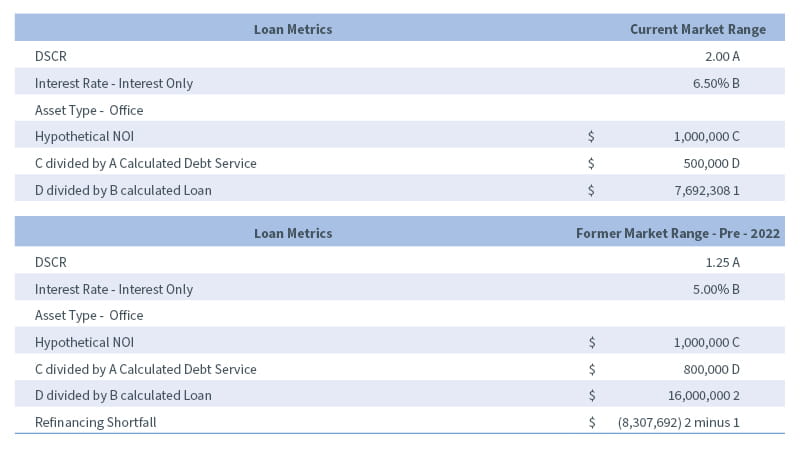
When the economy is struggling, lenders and investors are asking more from the real property. Therefore, lenders look to mitigate repayment risk and exposure by providing less loan proceeds, lower loan to values, and stronger covenant and DSCR requirements when originating new loans in the market. Alternatively, equity investors also pursue greater covenant protections, greater returns and controls on capital deployment, and ultimately pursue stricter conditions (limits) around the sponsor. For example, you might see a limit on sponsor fees, fund asset sales or transfers, demand for greater liquidity and net worth requirements, extensive financial reporting covenants, and dilution of ownership/loss of control. Basically, risk assessments around payback periods in today’s market create hurdles and boundaries that are not for the new investor or faint at heart.

Analysis of investment rate spreads above a risk-free rate

Proper analysis of financing market terms, and employment of the above capitalization rate techniques should not ignore other methods or analyses being used by peers and market participants. It is common practice for real estate analysts to compare historical spreads between U.S. Treasury rates (considered to be a risk-free-rate) and an expected market capitalization rate for a real estate investment. For investments with nearer-term investment horizons, we recommend analyzing risk-free rates with similar terms (for example: U.S. Treasury three-year rate, five-year rate, etc.). This comparison is intended to align investment risk with the respective hold period.

This begs the question: What do changes in reported investment rate spreads between published capitalization rates and the commonly used 10-year U.S. Treasury mean?

Typically, as risk-free rates increase, risk premium spreads correspondingly increase across the capital stack for a real estate investment. This concept follows a general premise known as positive leverage. Positive leverage occurs when equity yields on a real estate investment exceed the debt yield on the cost of debt used. Often, positive leverage is exhibited when the capitalization rate is greater than the debt’s stated interest rate. When the inverse of the above occurs, this is often referred to as negative leverage. As 10-year U.S. Treasury rates increase, investors seek returns greater than the U.S. Treasury rate for investments with similar hold horizons. Because real estate investments have a greater risk of loss, investors price in a wider (i.e., risk) spread to the risk-free rate and lock in returns/yields (using rate floors/minimum yields, origination and exit fees, and/or prepayment premiums) to create a return above the U.S. Treasury rate that will: (a) support the alternative (riskier) investment, and (b) support the associated asset management cost that exceeds lower-yield investments such as U.S. Treasuries. Ironically, this creates a negative impact on real property values. The real property must generate, or be able to generate, net operating income and net cash flow to generate both greater debt yields (interest rate) and equity yields (return) during recessionary periods and rising rates.

Market outlook

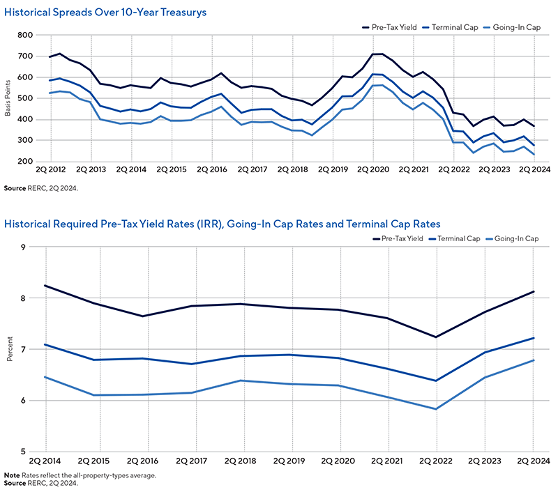
Simply, markets are not perfect and real estate is an illiquid investment, therefore real estate related market changes generally lag the public securities market. This is indicative of the charts below, and these charts imply that market participants may not believe current risk-free rates will hold over a longer-term period or continue to increase over a longer-term period, thus a justification for a tightening in the current risk premia spread. This suggests that longer-term rates (exit/reversion rates) may be equal to, or potentially less than, the going-in Cap Rate; Albeit, we are early in the cycle and this scenario has not yet occurred based on the below charts. 

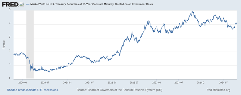
Taking the example from the Addenda in this article, the implied Cap Rate (Net Operating Income/Property Value) property data equates to 8.00%. As of the beginning of November 2024, the 10-year U.S. Treasury Rate (risk-free rate) is hovering around 4,321% which is higher than the long-term average of 4.25%. The difference between the risk-free rate and the implied Cap Rate is 382 basis points. This difference is above the historical spread (most recently 200 to 250 basis points) observed from Real Estate Research Corporation (RERC) data presented above, and the reasoning for the difference is that debt and equity investors are seeking higher yields in today’s environment, consistent with the previous discussion. 

Attributed to many positive U.S. based figures (not limited to strong employment and overall positive economic growth 2024 to date), we expect interest rates to normalize around historical levels rather than return to pre-COVID/2022 rates. Therefore, we anticipate a continued disconnect in value among willing buyers, willing sellers, and financing resources until the overall markets accepts that interest rates have normalized.

Concluding thoughts

Any of the above cap rate methods will produce a market-oriented answer. Depending on the level of information available, using one or reconciling between all three may be most appropriate.

In a perfect world, we’d suggest analyzing observable going-in rates from non-distressed and non-owner-occupier sales, and determining how leverage, equity yield requirements, or other real property and market-specific factors impacted the rate. Markets are imperfect, and in a volatile or distressed market, analysts and professionals must provide more thought and critical thinking to develop a market-based answer. 

Changing market conditions create complexity for an analyst. There isn’t a simple answer, but there are defined methods and a multitude of data resources available to today’s valuation professionals; all you need to do is go back to the basics. Go sharpen your #2 pencil, dust off the HP-12C sitting around your desk, and get to calculating so you can better answer and support today’s commercial real estate value.

Addenda

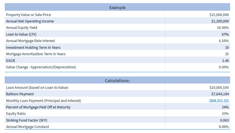
In the following section we present examples of how to use the computations discussed above. 

As an important clarification, the tables that follow (including the CR Excel Guide) are premised on a level payment stream for the amortization of debt. This may or may not be applicable depending on the market-based financing available.

Cap rate computations

The following table and related calculations from the preceding example reflect the previously discussed Cap Rate methods:

Strengths and weaknesses of each rate methodology

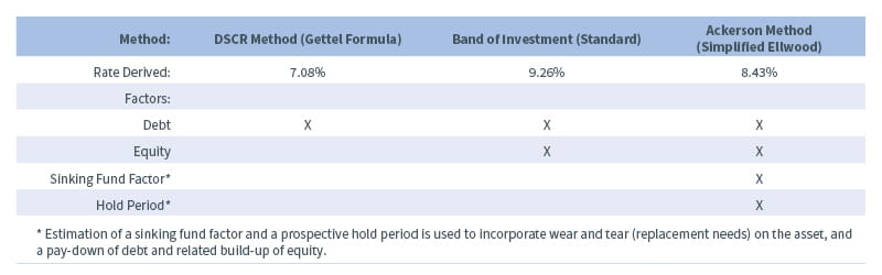
As shown in the table below, the DSCR method provides the lowest Cap Rate because it does not incorporate any equity yield. The Band of Investment (BOI) is the highest Cap Rate because it considers both debt and equity yields, but this method lacks any build-up of equity over an estimated hold period through amortization or value appreciation. The Ackerson Method, while the most complex, includes debt and equity components from the BOI as well as an estimate of equity build-up, estimated replacement needs, and any market-oriented estimate of appreciation or depreciation in market value.